Solving the Nerd-Sniping Problem: When Electronics meets Heat!

I recently stumbled upon this exciting problem from XKCD, aptly named as the Nerd-Sniping Problem:

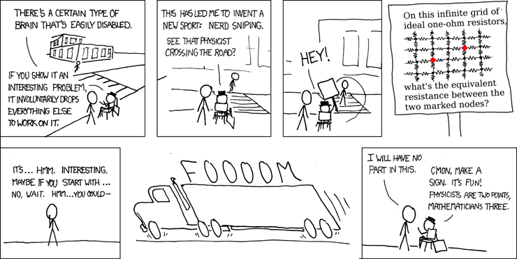
True to its name, it successfully managed to derail me from whatever it was that I was doing. The problem itself is quite curious, we have to find resistance between two points in an infinite lattice of ideal 1-ohm resistors.

Do not be fooled by the innocuous structure of the problem. It is, in fact, quite tricky, and true to its name, has the potential to Nerd-Snipe you. Being an empiricist through and through, I was curious if I could use some numerical methods to get a quick approximation for this particular problem. Something that immediately came to my mind was the Discrete Heat Equation in a 2D lattice and the structure of the problem seems similar enough to see if it applies here.

2D Heat Equation, as its name indicates, tells you how heat propagates in a 2D medium. Specifically, given that we know what’s the temperature in a conductor plate at some time t=0 is (aka the initial condition) and the temperature along the boundary, or some other points, which never changes, we want to predict how Heat propagates through the conductor and what is the temperature distribution like at any given moment in the future. The Heat Equation involves solving partial differential equations and is a tricky mathematical exercise, which we won’t be repeating here. Worth knowing, however, is the 2D Discrete Heat Equation.

In Discrete setting, we are typically given a lattice with some initial temperature conditions and are asked to derive how heat propagates at some discrete time-step in the future. For example, in the image below:

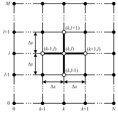
If we say that the temperature at the point (k, l) at timestep t is:

In simple words, the temperature at the mid-point is the average of all surrounding temperatures i.e. left, right, top, and bottom. Simple enough, right? Let’s see if we can use this idea for our resistance problem.

First, we start by seeing that Heat propagation and electric current flow are quite similar in nature. Heat transfers from point of high temperature to point of low temperature, when in contact. Current flows, similarly, from point of higher potential to that of lower potential. There is thermal conductivity (or resistivity) which works very similar to what electrical conductivity or resistivity works like. So, we have a compelling case for using the 2D Heat Equation for Electric Current propagation. Besides, if you consider Electric potential to be V(k,l) in a lattice, then you actually arrive at the same set of equations as above by using the KCL:

We first start by defining our problem:

N = 20                                # Assume a N x N grid
Grid = [[0.] * N for _ in range(N)]   # Initialize all potentials to 0

A = (N//2 - 1, N//2)                  # Point A
B = (N//2 + 1, N//2 - 1)              # Point B

def set(G, xy, v):
  x, y = xy
  G[x][y] = v

def get(G, xy):
  x, y = xy                          # Boundary has 0 potential
  if x < 0 or x > N-1 or y < 0 or y > N-1: return 0
  return G[x][y]

set(Grid, A, 100)                    # A has constant +100 V
set(Grid, B, -100)                   # B has constant -100 V

We consider a N x N grid with electric potential at each node to be 0. We then apply the potentials +100 to point A and -100 to point B (doesn’t have to be these exact numbers). Then we define functions that let us access any neighbors of a point in the lattice:

def left(xy):
  x, y = xy
  return x-1, y

def right(xy):
  x, y = xy
  return x+1, y

def top(xy):
  x, y = xy
  return x, y-1

def bottom(xy):
  x, y = xy
  return x, y+1

Next comes the main loop. For a fixed number of iterations, for each lattice point, we update it to the average of its four immediate neighbors.

def update(Grid, xy):
  x, y = xy
  # Get all neighbors
  l = left(xy)
  r = right(xy)
  t = top(xy)
  b = bottom(xy)
  # Take average
  four_pt = get(Grid, l) + get(Grid, r) + get(Grid, t) + get(Grid, b)
  four_pt /= 4
  # Update
  set(Grid, xy, four_pt)
  return

for epoch in range(500):
  for i in range(N):
    for j in range(N):
      S = (i, j)
      if S == A or S == B: 
        continue # we don't update these points, i.e. boundary cond.
      update(Grid, S)

A difference between the traditional Heat Flow setting is that it assumes some initial condition i.e. there is a certain temperature at certain place at the start. And a distinct boundary condition, i.e. the temperature at the boundary is always 0. But our initial conditions are simultaneously our boundary conditions as well. Which is to say, we assume that we have some potential at point A and B. But we also go on to assume that these potentials never change. Accordingly, we exclude these points from ever being updated in our code.

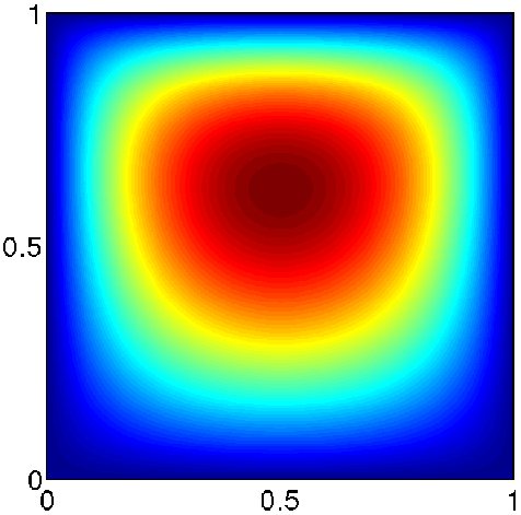
Before running our code, our initial grid looks as follows:

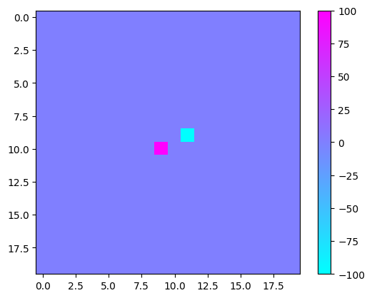
We have +100V potential at point A (lower left) and -100V potential at point B. After running our code for specified epochs, our final grid looks like:

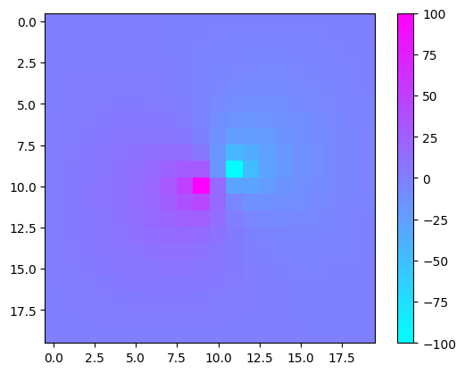
As you can see, the potential has been diffused because of current flow across different lattice points via the resistors. Once we have obtained the Electric potential across all points, obtaining the current flow at any lattice point is trivial. We just calculate all potential differences between the point and its neighbors and sum up the obtained currents. For the point B (the blue point with lower potential), we obtain total current flowing across it as:

current = get(Grid, left(B)) + get(Grid, right(B) ) + get(Grid, top(B) ) + get(Grid, bottom(B) ) - 4 * get(Grid, B)
# = 261.12551236325396

And once we have the net current entering node B, by Ohm’s law, the resistance between point A and point B must follow the relation:

In fact, we can repeat this calculation for multiple values of N and obtain the following chart:

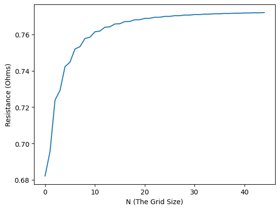
The values are clearly converging towards 0.77 ohms. And sure enough, the analytical result obtained for this problem exactly equals:

I hope you enjoyed this writeup! Be careful from Nerd-Sniping!! And do spread awareness about it by sharing this post!