Read my manifesto on Code as an alternative to Mathematics.
Code for this article can be found on this Colab Notebook should you choose to follow along.
Why Kalman Filters?
Kalman filters are ingenius. If you have never heard of them, then a very intuitive (and arguably reductive) way to think about them is to consider them as a funnel where you pour information from multiple noisy sources to condense them into a single more accurate statistic. Do not worry if all this sounds vague. In moments, we’ll be stripping that statement into a more accessible example in hopes of furthering our intuition. It is best said early that there is no better tool to study and reason about Kalman Filters than Mathematics. But it is equally true that the underlying Mathematics of Kalman Filters is challenging and has components of Linear Algebra, Probability Theory, and Calculus. As such, it may not be readily accessible to all. It is the objective of this article to hopefully provide you with an accessible intuition that’ll perhaps motivate you to dig deeper by yourself on this subject. And now, let’s start while keeping this in the back of our minds: “what follows is meant to provide intuition, and may not be entirely complete”.
Let’s get started by asking “why are Kalman Filters even necessary?” A simple, yet purposefully obtuse answer to this question is that real-life is not perfect. Consider this motivating example: Imagine a ship travelling in one dimension that leaves from the port (x=0) and travels for a bit. The Engine of the ship is configured to provide a constant velocity to the ship, of say 10m/s.
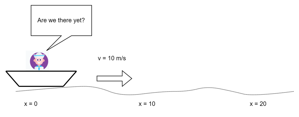
We begin by asking the question, where exactly is the ship 2 seconds after leaving the port? Naturally, you’ll say that the ship is at 2*10=20m distance away from the port because, after all, distance = velocity * time. And in an ideal world, this would indeed be true and there’d be no need for Kalman Filters at all. But, in real world, it’s never this simple. First, there may be no engine capable enough of producing force that causes the exact velocity of 10m/s at each point in time consistently. Sure enough, you may have the velocity of 10.00001 at some time or 9.99999 m/s or some number in between at other times but as is said, 99.99% perfect is still, at the end, imperfect. Secondly, even if you say that you indeed have such a perfect engine, it is never the case that when you apply a precisely measured force, you’ll have the intended perfect velocity. The wave motion can cause your ship to slow down just a tiny bit, or the wind can cause it to speed up, or who knows what can affect it in who knows what fashion.
Thus, you are never quite sure where your ship is at just by measuring where you wanted it to be.
Are we then doomed to never really know where we are at? Not quite! This is where sensors come in. Imagine that you, the sailor, have a GPS with you. The GPS is then able to precisely tell where you are at any given moment of time! In fact, you don’t even need the velocity of the ship now because no matter how the ship’s travelling, your GPS can always exactly tell you where you are. Problem solved? Like I said, not quite. In reality, sensors are often buggy and unreliable. Which is to say, they’ll indeed give you a measure of where you are, but the measure may not be precise. So, your GPS might tell you that at 3 seconds you are at 29.998 meters away from port or 30.002 meters, or even, and this is highly highly unlikely, 100 meters away from the port, but the point is that you can never fully rely on it. Additionally, you can never be sure that your sensor will never malfunction. Take for example the GPS sensor. The moment you find yourself in areas where there is no satellite coverage, it’s as good as non-functional. Indeed, if you had a sensor that you could guarantee never goes offline and measured what you wanted to know with an arbitrary degree of accuracy, there’d be no need for Kalman Filters at all.
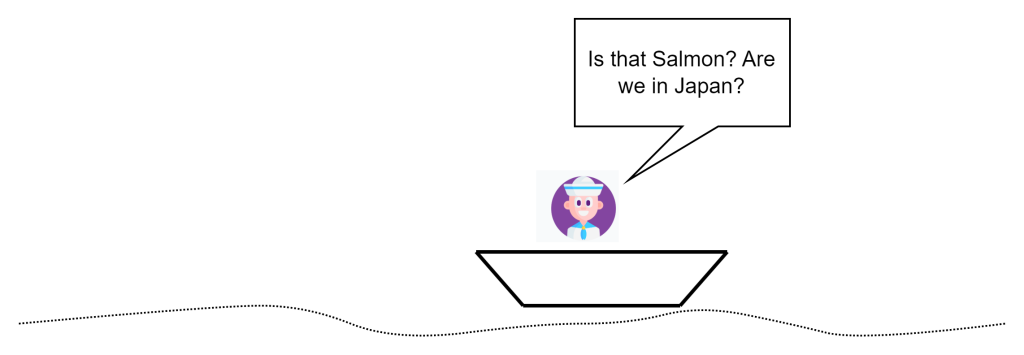
With this, we are now ready to answer why we need Kalman Filters. And the answer doesn’t really change from what we’ve already established earlier. A Kalman Filter is a funnel which takes two or more imperfect and unreliable information sources and generates a more accurate estimate of what you want to know. In this example, a Kalman Filter would take as input, your velocity estimate of where you are at any time, and your GPS estimate, if present, of where you are at that time, and then give you a more accurate estimate than both of those combined! And in fact, if you had more sources of information, like Radar, or Sonar, or even what kind of fish you currently see in the water, you could theoretically combine these measurements to produce an even more accurate estimate of your location.
Wait, where’s the maths?
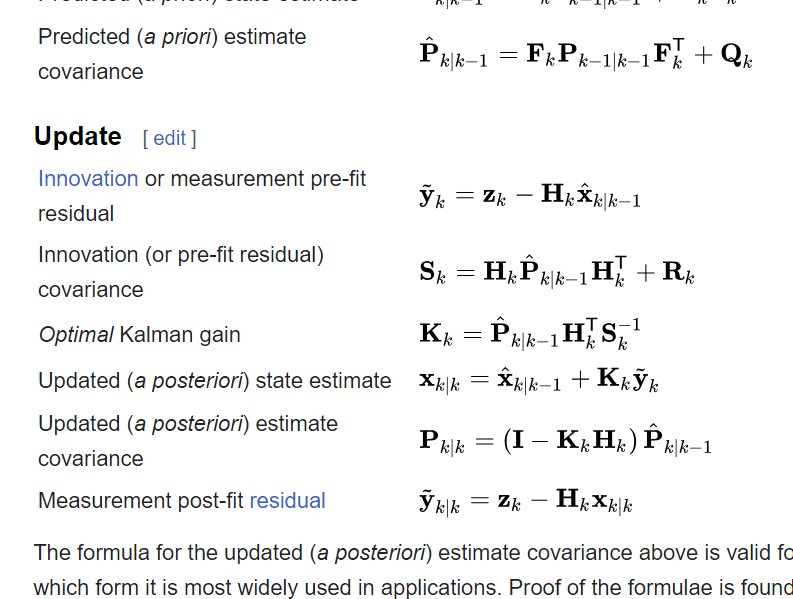
So, the question now is, how do we understand what Kalman Filter does and how it does it without using Mathematics such as this (from Wikipedia):
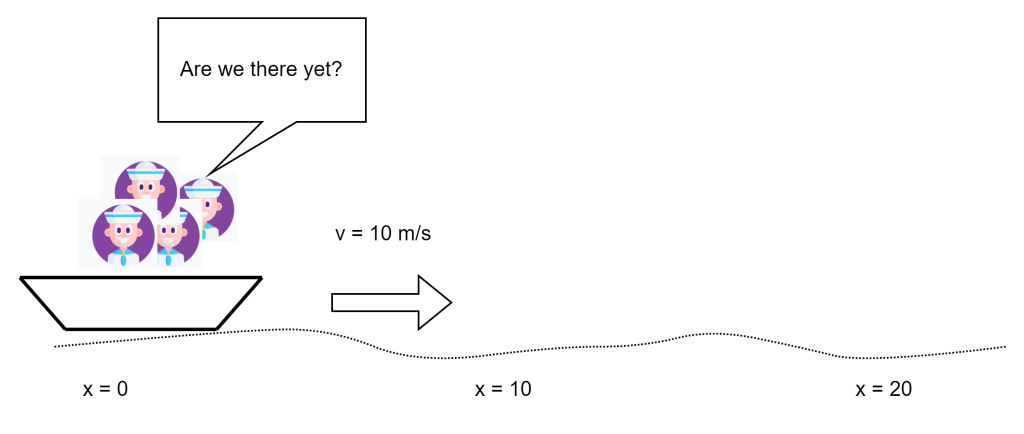
We start by assuming that instead of just one passenger, there are a thousand passengers on the ship, each with a GPS device of their own. Now, each passenger can estimate where they are (and consequently, where the ship is) by first doing a velocity-based estimation in the following fashion:
from random import gauss
def new_position(last):
  velocity = 10
  wind = gauss(0, 2)
  wave = gauss(0, 0.1)
  return last + velocity + wind + wave
Note: For an optional but more complete explanation of the gauss function, refer to the Appendix below. For now, it suffices to just say that it produces a random number (positive/negative) of the order indicated by the second parameter.
In essence, each of the 1000 passengers are doing thus: take the last known position (at the time before the present), add the velocity, and also, knowing that the wind and the water waves are going to slightly alter the course, add some random estimated fluctuations to it. Now if these passengers actually had good methods for estimating wind and water speeds, they’d use it. But since they don’t, they are estimating the effects by using random numbers. And truly, this is actually what happens in real life as well. We can’t measure everything, so we just estimate them using some simple methods like we did above with the mean (0) and the deviation parameters (0.1 and 2).
Now we are at the second phase of Kalman Filtering i.e. measurement. In this phase, all of the passengers, knowing that they only have an imperfect knowledge (owing to wind and water noise) of their state (where they are), seek to improve it using their sensors which works as such:
def sensor(t):
  if t == 3:
    # oops, passing through a thunderstorm. GPS fluctuating!
    sensor_noise = gauss(5, 10)
  elif t == 6:
    # uh-oh, satellite unavailable!
    sensor_noise = gauss(-5, 10)
  else:
    sensor_noise = gauss(0, 1)
  return true_position[t] + sensor_noise
Remember that sensors are imprecise equipments i.e. they do return mostly correct statistics, which in this case is the variable true_position, but they inherently have this noise which we are once again modelling by using a randomly generated number from the gauss function. Additionally, we are also modeling the unreliability of the sensor here by saying that at some instances (t=3 and t=6), the sensors are basically unavailable due to certain factors which are not at all inconceivable. So, every passenger, while using the sensor at any given time, will actually get different measurements.
A true Journey
Imagine, that this boat now leaves the port and travels these distances per second:
true_position = [0, 9, 19.2, 28, 38.1, 48.5, 57.2, 66.2,
                 77.5, 85, 95.2]
Which is to say, the ship starts from the port (x=0), and in the first second, travels 9 meters, in the second travels 10.2 meters and ends up at 19.2 meters and so on. The task of the passengers is to now predict, with the noisy and unreliable measurements that they have, these different positions at each second to as much accuracy as possible.
So, at time t = 1 a passenger may get these readings from the functions above:
# New position at t=1 if the last one t=0 was 0
new_position(0) => 9.37          (error -0.37)
# Sensor reading at t = 1s
sensor(1) => 8.98                (error +0.02)
And so on for all of the passengers. The question now remains, what’s the truth? Is our knowledge of Newtonian physics more reliable, or is the GPS sensor more reliable? In this particular case, since we already know that the true position of the boat is 9m from the true_position variable, the answer may be obvious, but this is not always the case. In such a scenario, to combine these two separate statistics, we actually resort to something quite simple: we take an average of the two! This actually ends up giving us, for the example above:
combined => (9.37+8.98)/2 => 9.17 (error -0.17)
Notice how the combined statistic has error less than the velocity estimate alone but is worse than sensor estimate for this example. But here’s the thing, we can actually do something better than taking the plain average. Consider the case where you know that your sensor is actually the state of the art and is pretty reliable. This would actually mean that you should favor what your sensor says more than what your velocity update is. You can actually do this by using something called a weighted average. Consider this code:
def combine(A, B, trustA, trustB):
  total_trust = trustA + trustB
  return (A * trustA + B * trustB) / total_trust
This combines two numbers from sources A and B but takes into account how much you trust these sources as well. So, if you call it as:
combine(9.37, 8.98, 10, 1) => 9.33         (error -0.33)
combine(9.37, 8.98, 1, 10) => 9.01         (error -0.01)
In the first call, you trust source A (velocity) much more than source B (sensor) i.e. 10 vs 1 so the answer you get gravitates towards source A i.e. is closer to 9.37. Whereas, in the second call, it’s actually the reverse and the answer gravitates towards source B. This trust based weighted averaging is the heart of the Kalman filter and this is what gives it its data combining power.
But now, we are presented with a new question. Which source is more trustworthy or how do you calculate the trust? Should velocity be favored? Or should GPS measurements be favored? That which decides this is the deviation or the variance metric. Think about it, what’s more trustworthy? An information source that fluctuates wildly or one that doesn’t? To put it into perspective, imagine that you tune into 10 weather radio stations, 4 out of them tell you that it’s going to rain and 6 out of them tell you that it’s going to be sunny. Now imagine that you log into 10 weather websites and 9 out of them tell you that it’s going to rain, and 1 tells you that it’s going to be sunny. Which source is more reliable here? Are you inclined to believe what majority of weather radio stations tell you (sunny)? Or are you inclined to believe what weather websites tell you (rainy)? A rational course of action is to favor the conclusion of the websites more because many of them are in agreement with the conclusion i.e. they have low variance whereas weather radio stations, at least in this example, appear to fluctuate wildly in their conclusions, so perhaps shouldn’t be trusted too much.
The complete update step then becomes as such:
from statistics import variance

# Find updated positions per passenger at t seconds
def update(t, last):
  velocity_updates = []
  sensor_updates = []

  for p in range(1000):   # for each passenger
    # new velocity update based on last known position
    # for the passenger
    velocity_updates.append(new_position(last[p]))
    sensor_updates.append(sensor(t))

  # Calculate trust metrics for velocity and sensor measurements
  # Remember that as fluctuation increases, trust decreases
  # And vice-versa
  fluctuation_velocity = variance(velocity_updates)
  fluctuation_sensor = variance(sensor_updates)

  # calculate trust
  trust_velocity = 1/fluctuation_velocity
  trust_sensor = 1/fluctuation_sensor

  # combine these together for each passenger
  combined = []
  for p in range(1000):
    combined.append(combine(A = velocity_updates[p],
                            B = sensor_updates[p],
                            trustA = trust_velocity,
                            trustB = trust_sensor))
  # Sensor updates & velocity updates returned for plotting purposes
  return sensor_updates, velocity_updates, combined
Note: More on the Variance function in the Appendix. For now, just consider it as a measure of the fluctuations in a list of numbers.
This code is relatively straightforward. For each passenger, it’s doing the noisy velocity-based measurement and a noisy sensor-based measurement. Based on these measurements for all of the passengers, it’s then calculating a trust metric for each of these measurements as inverse of variance (because as variance increases, trust decreases), and then calling the combine method with relevant trust parameters. It is important to note that each passenger here is doing a location update for themselves. At the end of such individual updates, the actual location of the ship itself can be inferred as the average of all passenger locations.
Results
To tie the entire code presented above, we use the following code.
# We'll do a final plot using this list
plot_data = []

def update_plot(t, sensor, velocity, combined_position):
  # add true position at this time
  plot_data.append({'passenger': 'true', 'type': 'true', 'time': t,
                    'position': true_position[t]})
  # for each passengers
  for p in range(1000):
    plot_data.append({'passenger': p, 'type': 'sensor', 'time': t,
                    'position': sensor[p]})
    plot_data.append({'passenger': p, 'type': 'velocity', 'time': t,
                    'position': velocity[p]})
    plot_data.append({'passenger': p, 'type': 'combined', 'time': t,
                    'position': combined_position[p]})

update_plot(0, [0]*1000, [0]*1000, [0]*1000)
estimated_positions = [0]*1000    # all estimates start from 0
for t in range(1, 10):   # ten seconds
  _sensor, _velocity, estimated_positions = update(t, estimated_positions)
  update_plot(t, _sensor, _velocity, estimated_positions)
The update_plot function just does basic book-keeping to store transient statistics for plotting purposes. The main iteration here is simply the bottom-most for loop which, continuously updates position estimates at any given time by using current best estimates that a passenger has. Apart from these, the code is essentially self-explanatory.
When plotted using the seaborn library, you can see the following results:
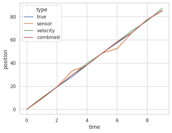
Which is a bit difficult to parse due to the present scale. Let’s zoom into these two areas in particular t=0.75 to t=1 i.e. when the sensor is functioning properly, and t=2 to t=4, when there is a glitch.
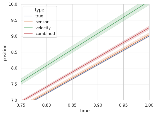
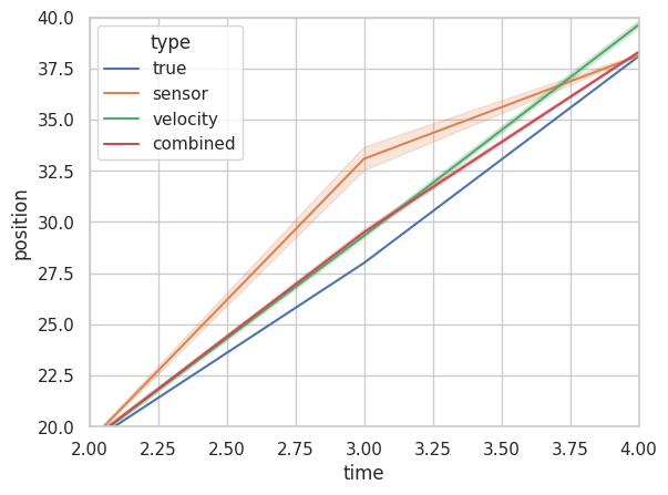
Note: The envelope refers to uncertainty. The wider the envelope in the line, the more uncertain we are about the number.
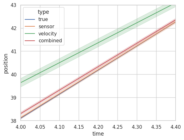
In the first case, as you can see, the combined position estimate of all 1000 passengers is better than just the velocity estimate alone (in green) and while our estimate is indeed worse than our sensor readings in the first case, in the second case we actually do a lot better than our malfunctioned sensor reading alone! This is because Kalman Filter automatically adjusts for wild variations caused by unforeseen fluctuations and always provides us with a reasonably reliable metric. As you can see in the figure below, once our sensors recover (t=4 to t=5), Kalman Filter starts favoring the sensors once again (bit difficult to see because sensor reading and true value overlap so much).
Conclusion and Remarks
I’d like to believe that you got at least some intuition about how Kalman Filters work. The actual theoretical foundations of Kalman Filters are equally intriguing and I encourage you to pursue it further if your work requires it. Meanwhile, I hope that this demonstrates just how much Code as a formal language can help impart intuitions to concepts that, at first glance, can come off as daunting. I also hope to be able to impart a few more insights into topics that I find fascinating with the help of simple code.
Appendix
The Gauss function
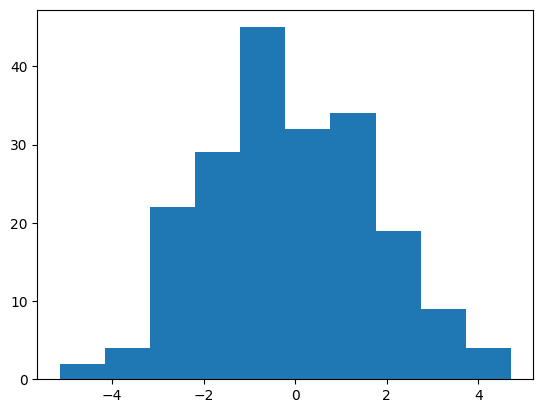
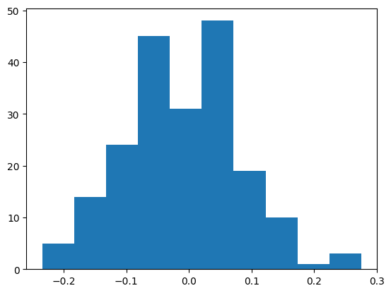
The only special function you need to know here is the normal distribution function i.e. gauss(0, 0.1) and gauss(0, 2). Simply put, it gives you a random number, which is most often near 0 (the technically correct way to say this is that it’s centered around 0) and the chances of getting a number farther away from 0 is controlled by the second parameter i.e. 2 and 0.1.
So, if you call gauss(0,0.1), you are more likely to get numbers such as 0.06, -0.07, -0.06, 0.02, -0.23, -0.06, 0.09, etc in no particular order.
Whereas if you call gauss(0, 2), you are more likely to get numbers such as 1.05, 1.03, -1.06, 0.32, 1.29, -0.40, -1.72 etc, again, in no particular order.
Intuitively speaking, the second parameter, also called the standard deviation, controls how much what you’re measuring fluctuates. In the code above, this means that you generally expect wind to deviate too much (windy day?) and water waves to deviate less (calm waters). Notice in the histogram below how often a number is produced by deviation=2, and deviation=0.1 (pay special attention to the x-axis). Although the range of numbers are quite different, the shape of both of these histograms look about the same. This tell-tale bell-like shape is called Gaussian or Normal or Bell Curve distribution and if occurs quite often in nature.
Variance
Variance is a measure of consistency. Which is to say, if you are consistent, you have low variance and vice versa. In the figure above, you can’t quite see the variance because the x-axes are actually adjusted automatically. If we were to plot the histogram above within the same axes limits, we would get something like this:
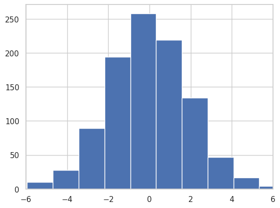
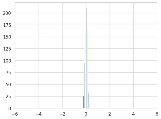
Notice how the first image is wider? That’s because the numbers vary quite a lot in it. Which is to say, you expect to find lots of -2s, 2s, 0s, and some 4s, -4s in it. But in the second image, you would expect to find lots of 0s and 0.1s, -0.1s etc, but you would expect a lot less of -2, 2 etc. To be correct, the first distribution has a higher variance (4 to be precise) than the second which only has (0.01). More information on Variance can be found online.